Decision Trees (DT)

Geometric Intuition of Decision Trees: Axis-Parallel Hyperplanes

A Decision Tree is a flowchart-like structure that recursively splits data based on feature values. Each split creates decision boundaries that are parallel to the feature axes, which makes decision trees highly interpretable. Below, we explore how a decision tree models the given dataset.

Dataset Used

This dataset contains four predictor variables (Outlook, Temperature, Humidity, and Windy) and a target variable (Play Golf?), which the decision tree uses to classify whether playing golf is feasible or not.

How the Decision Tree Works on This Dataset

1. Step 1: Splitting on Outlook (First Decision Boundary)
   • The tree first checks Outlook because it is the most informative feature.
   • This results in three distinct groups in the feature space:
     • If Outlook = Overcast → Always "Yes" (No further splitting needed).
     • If Outlook = Sunny → Further splits occur based on Windy.
     • If Outlook = Rainy → Further splits occur based on Humidity.
2. Step 2: Further Splitting on Other Features
   • For Sunny Days:
     • If it is Windy = False → "Yes" (can play golf).
     • If it is Windy = True → "No" (not suitable).
   • For Rainy Days:
     • If Humidity = High → "No" (too humid to play).
     • If Humidity = Normal → "Yes" (good conditions).
3. Final Decision Boundaries
   • The dataset is now divided into smaller rectangular decision regions, each corresponding to a final classification (Yes/No).
   • Each leaf node in the decision tree represents a final classification for a set of feature values.

Geometric Intuition: How the Tree Creates Decision Boundaries

• The decision tree divides the feature space into axis-parallel regions.
• Each split corresponds to a vertical or horizontal boundary in the space of selected features.
• The resulting decision regions are rectangular and aligned with feature axes.
• This structure is different from models like logistic regression, which create diagonal decision boundaries.

Example: Decision Boundaries for Outlook & Humidity

If we visualize a 2D feature space with Outlook on the x-axis and Humidity on the y-axis:

• The first split at Outlook = Overcast creates a vertical boundary separating "Yes" from the rest.
• The second split at Humidity = High for Rainy days creates a horizontal boundary in the Rainy region.
• Further splits (like Windy for Sunny days) refine the classification into more rectangular segments.

Key Takeaways

• ✅ Decision Trees create axis-aligned decision boundaries (rectangular regions).
• ✅ Each split represents an IF-ELSE condition, forming nested rules.
• ✅ Deeper trees create more refined partitions, improving accuracy but risking overfitting.

This makes Decision Trees intuitive and interpretable, but they may struggle when dealing with complex, non-rectangular patterns in data. Would you like a visual example of the decision regions? 🚀

Explain Entropy?

Entropy

• Entropy is a measure of unpredictability. A feature with higher entropy has more random values than the one with lower entropy.
• Suppose we tossed a coin 4 times,

• For a given random variable Y which has K values, then entropy of Y is:

• For example, for the above play golf example, there are two classes:

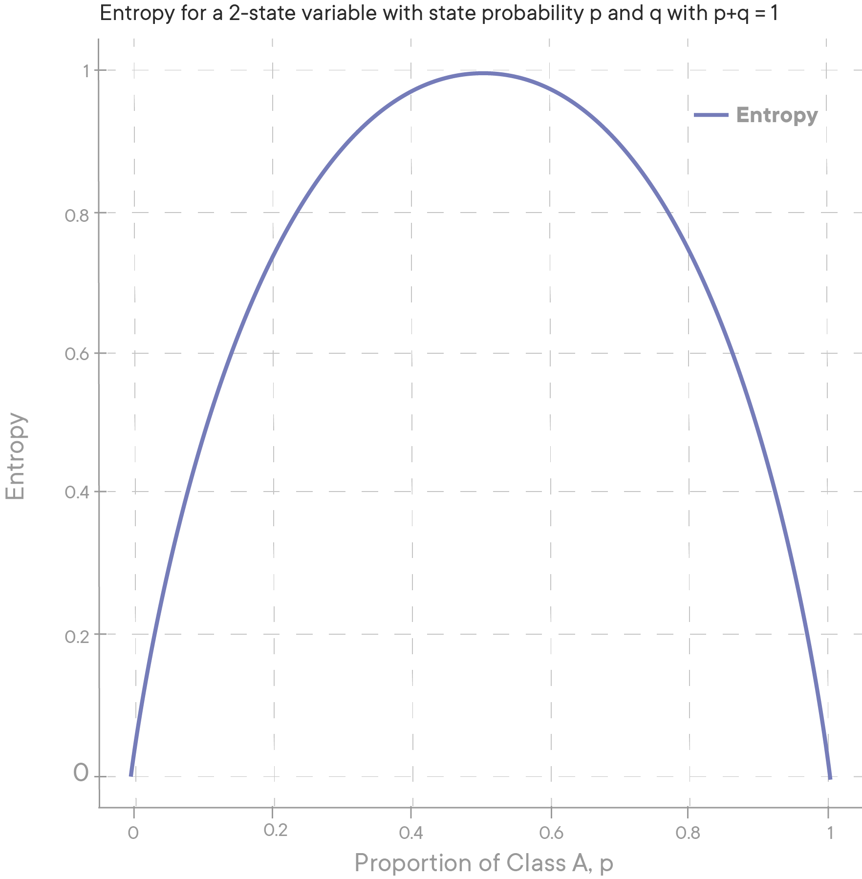
Comparing entropies for different cases for 2-class example

Sr. No.	P(Y+)	P(Y-)	Entropy
1	99%	1%	0.08
2	50%	50%	1.00
3	100%	0%	0.00

If both classes are equally probable, we have a maximum entropy value of 1.

If one class fully dominates, the entropy value becomes 0.

Comparing entropies for different cases for Multi-class example

• If all classes are equiprobable, the entropy will be maximum, i.e., uniform distribution.

• If one class has 100% probability and others are zero, the entropy is minimum.
• In this figure, entropy of skewed distribution will be lesser than that of normally distributed. More peaked is the distribution, lesser will be the entropy.

• Kullback-Leibler Divergence or relative entropy

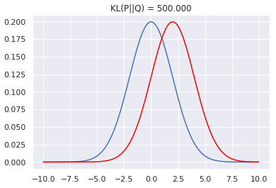
• KL Divergence measures the difference between two probability distributions over the same variable X.
• For Discrete probability distributions P & Q on the same probability space X

\( D_{KL}(P || Q) = \sum_{x \in X} p(x) \log \frac{p(x)}{q(x)} \)

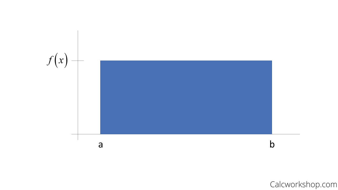
• For distributions P and Q of a continuous random variable

\( D_{KL}(P || Q) = \int_{-\infty}^{\infty} p(x) \log \frac{p(x)}{q(x)} \,dx \)

p(x) and q(x) are probability densities of P & Q

Explain Information Gain

                          Outlook
                          //   ||  \\
                                ________//    ||   \\_____________
                                |            |                |
                             Sunny         Overcast          Rainy
                               |              |               |
                              Windy        Play=Yes          Humidity
                            ____|____                     ____|____
                            |        |                    |         |
                          False    True                High      Normal
                        Play=Yes  Play=No           Play=No    Play=Yes